1s = 1 000 ms (10^3 millisecond)
1s = 1 000 000 000 ns (10^9 nanosecond)

// operazioni in memoria, sostanzialmente estantanee
L1 cache reference 0.5 ns
Branch mispredict 5 ns
L2 cache reference 7 ns
Main memory reference 100 ns


Compress 1K bytes with Zippy 3ms
Send 2K bytes over 1 Gbps network 0,2 ms
Read 1 MB sequentially from memory 0,25 ms
Round trip within same datacenter 0,5 ms
Disk seek 10 ms
Read 1 MB sequentially from disk 20 ms
Send packet CA->Netherlands->CA 150 ms

1 query select su indice 1ms
back-of-the-envelop con quantità notevoli
How long to generate image results page (30 thumbnails)?
Design 1: Read serially, thumbnail 256K images on the fly
  30 seeks * 10 ms/seek + 30 * 256K / 30 MB/s = 560 ms
Design 2: Issue reads in parallel:
  10 ms/seek + 256K read / 30 MB/s = 18 ms
(Ignores variance, so really more like 30-60 ms, probably)
Lots of variations:
– caching (single images? whole sets of thumbnails?)
– pre-computing thumbnails
Il metodo standard per affrontare il problema della prestazione di un algoritmo è detto "big-O notation".
la notazione Big-O si riferisce ad una performance RELATIVA, ad esempio, anziche misurare in quanto tempo un algoritmo esegue il suo compito big-O specifica come si comporta l'algoritmo quando il suo imput cresce. big-O specifica la relazione(come una funzione matematica) tra il tempo di esecuzione di un algoritmo e la grandezza dell'imput. se ad esempio un algoritmo di ordinamento impiega 50ms per 500elementi e 100ms per 1000 elementi, la sua performance è detta lineare, perchè il tempo cresce proporzionalmente all'imput, si esprime con la notazione 0(n), dove 0 significa che stai usando la notazione big-O e n rappresenta la grandezza dell'input. purtroppo non tutti gli algoritmi hanno performance lineare...
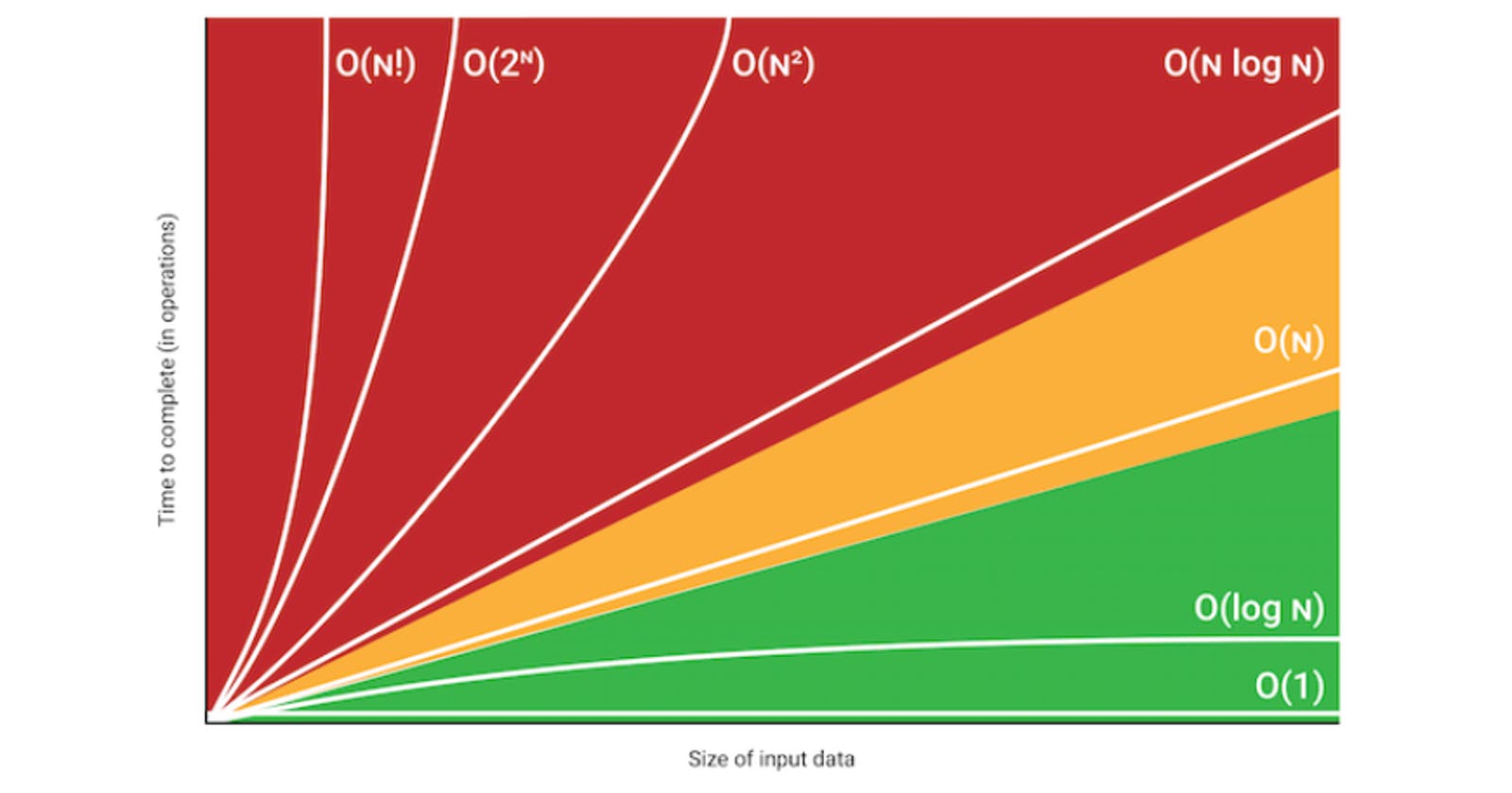
alcune notazioni standard, dalle più favorevoli alle peggiori:
 Algorithm Complexity           Big-O Notation       Explanation                      Example Algorithms
      Constant                       O(1)                 Running time is inde-           es. Accessing a single element in an array, is independent of input size.
      Logarithmic                    O(log n)             The running time is a  function of the logarithm base 2 of the input size.          es. Finding an element in a sorted list using binary search


      Linear                         O(n)                 The running time is directly proportional to the input size.        es. Finding an element in an unsorted list


      Linear Logarithmic             O(n log n)           The running time is a function of the linear times the logarithmic functions of the input size        es.  Merge sort

      Quadratic   O(n2)                                        The running time is a function of the square algorithm like  of the input size      es.    A slower sorting selection sort
tuttavia big-O non è sufficiente a descrivere le prestazioni di un algoritmo(che potrebbe essere molto lento e scalare bene), ma serve a capire quanto bene quell'algoritmo scala su grosse quantità di dati. . se due algoritmi dichiarano di scalare con la stessa progressione, ad esempio O(n log n), questo non dice quale dei due algoritmi sia effettivamente più veloce, occorrono test mirati
ancora, quando l'input è di piccole dimensioni, un algoritmo che non scala bene potrebbe essere più veloce
Notation   Name         Example
O(1)       constant     array index
O(1ogn)    logarithmic  binary search
O(n)       linear       string comparison
O(n1ogn)   nlogn        quicksort
0(n2)      quadratic    simple sorting methods
o(h3)      cubic        matrix multiplication
O(2")      exponential  set partitioning
Accessing an item in an array is a constant-time or O(1) operation. An algorithm that eliminates half the input at each stage, like binary search, will generally take O(1ogn). Comparing two n-character strings with strcmp is O(n). The traditional matrix multiplication algorithm takes 0 ( n 3 ) , since each element of the output is the result of multiplying n pairs and adding them up, and there are n2 elements in each matrix. Exponential-time algorithms are often the result of evaluating all possibilities: there are 2" subsets of a set of n items, so an algorithm that requires looking at all subsets will be exponential or O(2"). Exponential algorithms are generally too expensive unless n is very small, since adding one item to the problem doubles the running time. Unfortunately there are many problems, such as the famous "Traveling Salesman Problem," for which only exponential algorithms are known. When that is the case. algorithms that find approximations to the best answer are often substituted.
O(1) describes an algorithm that will always execute in the same time (or space) regardless of the size of the input data set.
bool IsFirstElementNull(String[] strings)
{
    if(strings[0] == null)
    {
        return true;
    }
    return false;
}
O(N) describes an algorithm whose performance will grow linearly and in direct proportion to the size of the input data set. The example below also demonstrates how Big O favours the worst-case performance scenario; a matching string could be found during any iteration of the for loop and the function would return early, but Big O notation will always assume the upper limit where the algorithm will perform the maximum number of iterations.
bool ContainsValue(String[] strings, String value)
{
    for(int i = 0; i < strings.Length; i++)
    {
        if(strings[i] == value)
        {
            return true;
        }
    }
    return false;
}
O(N2) represents an algorithm whose performance is directly proportional to the square of the size of the input data set. This is common with algorithms that involve nested iterations over the data set. Deeper nested iterations will result in O(N3), O(N4) etc.
bool ContainsDuplicates(String[] strings)
{
    for(int i = 0; i < strings.Length; i++)
    {
        for(int j = 0; j < strings.Length; j++)
        {
            if(i == j) // Don't compare with self
            {
                continue;
            }

            if(strings[i] == strings[j])
            {
                return true;
            }
        }
    }
    return false;
}
O(2N) denotes an algorithm whose growth will double with each additional element in the input data set. The execution time of an O(2N) function will quickly become very large.
bool ContainsValue(String[] strings, String value)
{
    for(int i = 0; i < strings.Length; i++){ // first elaboration
    }
    for(int i = 0; i < strings.Length; i++){ // seccond elaboration
    }
    return false;
}
Logarithms are slightly trickier to explain so I'll use a common example: Binary search is a technique used to search sorted data sets. It works by selecting the middle element of the data set, essentially the median, and compares it against a target value. If the values match it will return success. If the target value is higher than the value of the probe element it will take the upper half of the data set and perform the same operation against it. Likewise, if the target value is lower than the value of the probe element it will perform the operation against the lower half. It will continue to halve the data set with each iteration until the value has been found or until it can no longer split the data set. This type of algorithm is described as O(log N). The iterative halving of data sets described in the binary search example produces a growth curve that peaks at the beginning and slowly flattens out as the size of the data sets increase e.g. an input data set containing 10 items takes one second to complete, a data set containing 100 items takes two seconds, and a data set containing 1000 items will take three seconds. Doubling the size of the input data set has little effect on its growth as after a single iteration of the algorithm the data set will be halved and therefore on a par with an input data set half the size. This makes algorithms like binary search extremely efficient when dealing with large data sets.
logarithm of a number to a given base is the power or exponent to which the base must be raised in order to produce the number.
x = base^y == y = log(x)
http://science.slc.edu/~jmarshall/courses/2002/spring/cs50/BigO/index.html

associative arrays are implemented as hash tables - so lookup by key (and correspondingly, array_key_exists) is O(1) However, arrays aren't indexed by value, so the only way in the general case to discover whether a value exists in the array is a linear search O(n).
Most of the functions you're curious about are probably O(n).
test for presence using isset($large_prime_array[$number]). it's in the order of being hundreds of times faster than the in_array function.
Interesting Points:
isset/array_key_exists is much faster than in_array and array_search
+(union) is a bit faster than array_merge (and looks nicer). But it does work differently so keep that in mind.
shuffle is on the same Big-O tier as array_rand
array_pop/array_push is faster than array_shift/array_unshift due to re-index penalty
Lookups:

array_key_exists O(n) but really close to O(1) - this is because of linear polling in collisions, but because the chance of collisions is very small, the coefficient is also very small. I find you treat hash lookups as O(1) to give a more realistic big-O. For example the different between N=1000 and N=100000 is only about 50% slow down.

isset( $array[$index] ) O(n) but really close to O(1) - it uses the same lookup as array_key_exists. Since it's language construct, will cache the lookup if the key is hardcoded, resulting in speed up in cases where the same key is used repeatedly.

in_array (n) - this is because it does a linear search though the array until it finds the value.

array_search O(n) - it uses the same core function as in_array but returns value.

Queue functions:

array_push O(∑ var_i, for all i)

array_pop O(1)

array_shift O(n) - it has to reindex all the keys

array_unshift O(n + ∑ var_i, for all i) - it has to reindex all the keys

Array Intersection, Union, Subtraction:

array_intersect_key if intersection 100% do O(Max(param_i_size)*∑param_i_count, for all i), if intersection 0% intersect O(∑param_i_size, for all i)

array_intersect if intersection 100% do O(n^2*∑param_i_count, for all i), if intersection 0% intersect O(n^2)

array_intersect_assoc if intersection 100% do O(Max(param_i_size)*∑param_i_count, for all i), if intersection 0% intersect O(∑param_i_size, for all i)

array_diff O(π param_i_size, for all i) - That's product of all the param_sizes

array_diff_key O(∑ param_i_size, for i != 1) - this is because we don't need to iterate over the first array.

array_merge O( ∑ array_i, i != 1 ) - doesn't need to iterate over the first array

+ (union) O(n), where n is size of the 2nd array (ie array_first + array_second) - less overhead than array_merge since it doesn't have to renumber

array_replace O( ∑ array_i, for all i )

Random:

shuffle O(n)

array_rand O(n) - Requires a linear poll.

Obvious Big-O:

array_fill O(n)

array_fill_keys O(n)

range O(n)

array_splice O(offset + length)

array_slice O(offset + length) or O(n) if length = NULL

array_keys O(n)

array_values O(n)

array_reverse O(n)

array_pad O(pad_size)

array_flip O(n)

array_sum O(n)

array_product O(n)

array_reduce O(n)

array_filter O(n)

array_map O(n)

array_chunk O(n)

array_combine O(n)
#include <set>
#include <map>
#include <hash_map>

map<key, value>
hash_map<key, value>
A Hash Map (or other data structure using a hashing algorithm) is extremely quick in terms of access time. It is O(1) constant time regardless of input size; basically instantaneous.
There is a flip side to this however. A Hash Map does not sort the data in any way. So if you need to keep your data in some kind of order, you will have to stick with std::map, which has O( log n ) access time, or some other data structure.
Partita Iva: 02360450205
Content of this site is licensed under Creative Commons Attribution-Share Alike License.